Theory

---

Processing

---

Linear prediction

Linear prediction estimates the value of a point based on the values of adjacent points. This method can be used to replace corrupted values in an FID. For example, in NMR experiments with fast relaxation rates, data collection must begin almost immediately following an RF pulse, even before the receiver and preamplifier can fully recover from ringing and saturation caused by the RF pulse. Consequently, several of the first datapoint values can be corrupted by instrumentation-induced noise. The effect of this noise on the spectrum can be profound because it often amounts to large fractions of the highest-amplitude signal values. Therefore the spectrum can improve noticeably when these corrupted point values are replaced with values estimated by linear prediction, where the estimated values are based on subsequent points of greater integrity.

A second application of linear prediction to NMR data is to extend an FID. This is useful for experiments in which data collection ceased before the signals completely decayed; that is, the FID is truncated. Here, the data values of the FID are used to estimate new data values that are appended to the end of the FID. Often the FID can be extended 20% or more by this means.

The Process1D/Transform/Linear Prediction menu item uses linear prediction to replace data values at the beginning or end of the FID and can also be used to extend the FID. The mathematical underpinnings of the linear prediction algorithm are discussed next, so that in the ensuing descriptions of the menu items, the settings in the control panels may be related to the mechanics of the algorithm.

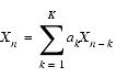
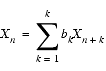
Forward prediction is based on the assertion that the value of the nth data point X_n is determined from the values of K antecedent points:

Eq. 1

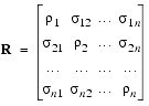
where a_k are the linear prediction (LP) coefficients. These LP coefficients are determined from n-k values of X_n, cast in matrix notation as:

Eq. 2

In general, the matrix C is over-determined; therefore, the solution to this equation is found by least-squares analysis, which is based on a singular value decomposition in order to ensure a solution when C^TC is not invertible:

Eq. 3

The matrices n, L, and u are obtained from the singular value decomposition of the matrix C. The matrix L is a diagonal matrix of singular values of the columns of n and u containing the right and left singular vectors.

With knowledge of the maximum number of signals in the FID, the number of singular values in the matrix L can be reduced by truncating the matrices n, L^-1, and uT. The result is reduced noise in the predicted points (Makhoul 1978, Kumaresan and Tufts 1982, Barkhuijsen et al. 1985).

To assure that the predicted data points are well behaved, i.e. decaying, the technique of "root reflection" is often used. In this procedure, one constructs a complex polynomial defined by the LP coefficients. Then the roots are determined from this polynomial. For a noiseless FID, the roots should lie within the unit circle, which, of course, does not always hold for real data. To enforce proper behaviors, one reflects all the roots into the unit circle and reconstructs the polynomial from which a new set of LP coefficients are extracted (see e.g., Zhu and Bax 1993).

For backward linear prediction, you start with an analogous linear equation, as in Eq. 1:

Eq. 4

The mathematics of determining b_k are similar to that used for forward prediction. However, you must pay attention when using root reflection that the roots in this case are reflected outside the unit circle.

Lastly, as pointed out by Zhu and Bax (1993), it is sometimes advantageous to perform both backward and forward predictions to obtain averaged LP coefficients. This procedure tends to be very good at suppressing noise and artifacts.

As mentioned earlier, linear prediction is accessed using the Process1D/Transform/Linear Prediction command. Choosing this displays a control panel. The following three controls, which determine how the LP calculation is performed are set in the control panels: Points to use, Number of coefficients, and Number of peaks. Points to use defines the number of points used to calculate the LP coefficients a_k or b_k. This corresponds to the value n in Eq. 1. The Number of coefficients corresponds to the value n-k. And Number of peaks is used to truncate the matrices n, L, and u (Eq. 3).

---

Automatic phase correction

FELIX has several alternative autophasing methods for 1D spectra and one method for 2D and 3D spectra. The basic method and the method based on peak integration are used exclusively for 1D spectra. The method based on PAMPAS (Dzakula 1999) or APSL (Heuer 1991) is commonly used for 1D, 2D, and 3D spectra and is described in this section.

For a 1D spectrum in the workspace or a selected dimension of an ND spectrum, FELIX divides the spectrum into 10-40 segments of equal widths along the phasing dimension and tries to find a best sample peak per segment. The phase error of each individual sample peak is detected using the PAMPAS or APSL algorithm, and then the global zero- and first-order phase errors (represented by FELIX symbols phase0 and phase1) are obtained by linear regression analysis.

If solvent peaks or other noise peaks exist in the spectrum, it is important to exclude them from the phase detection process. FELIX allows you to define up to 10 excluded areas (using the aph exclude command). An excluded region is specified by the starting and ending datapoint numbers, and the dimension if it is an ND spectrum (which can be different from the phasing dimension). Any peaks that fall in the specified range along this dimension are not used as sample peaks.

For an ND spectrum, FELIX searches all the vectors along the phasing dimension and tries to find a best sample peak for each segment, without considering peaks in the excluded areas. Peaks are selected based on their width (must be wider than a user-defined threshold), height (the higher the better), and symmetry (the more symmetric the better). For a 1D spectrum, sample peaks are searched similarly in the only vector for each segment.

If more than two sample peaks are found for the whole spectrum, the phase errors are detected from each of them. Next, the global phase parameters (phase0 and phase1) are obtained by linear regression analysis. The phase errors detected are between 0° and 180°, which do not reflect the actual phase differences between them. The possible p-jumps between the individual phase errors are automatically compensated within the expected range of phase1. The default range of phase1 is approximately -720° to 720°. You can change the range of phase1 when using the aph command. See FELIX Command Language Reference for more details about using this command.

---

Assign

---

Basis of the assignment strategy

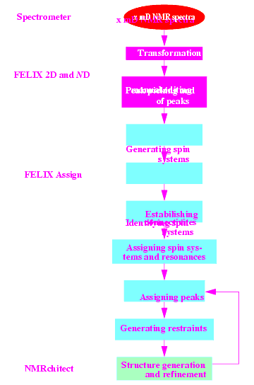
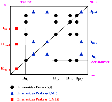
One approach to making assignments, developed by Wüthrich and coworkers (Wüthrich 1986), is the "sequential assignment strategy", which obtains sequence-specific resonance assignments (see following figure).

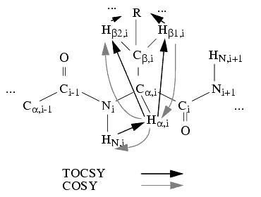
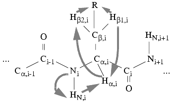
The first step in this procedure is the delineation of individual spin systems, based on homonuclear 2D and/or 3D spectra or on heteronuclear spectra. If homonuclear 2D spectra are utilized, this spin-system delineation can be based on COSY type spectra (e.g., DQF-COSY or P-COSY). A spin system is understood to be a group of spins connected by scalar or through bond spin-spin couplings. This means that, for homonuclear spectra of a peptide or protein, one amino acid residue can contain one or more spin systems. However, due to the peptide bond (which yields a structure in which no non-labile hydrogens are three bonds apart in neighbor residues) spin systems do not comprise spins from more than one residue. Therefore, in a COSY-type spectrum, cross peaks are expected between scalarly coupled spins within individual residues.

For spin-system delineation, the TOCSY or HOHAHA type spectra can also be used, since the cross peaks arise only within individual spin systems. Ideally, TOCSY contains more cross peaks for the same spin system than COSY; thus, in complicated overlapping situations it is advantageous to combine the information from both types of spectra.

For spin-system delineation or detection it is possible to use two different methods: systematic searching (when all the spin systems in the spectrum are collected through systematically searching the spectrum for well-aligned peaks) and simulated annealing.

The complete delineation of spin systems is facilitated by the fact that the chemical shifts of the protons are in well defined regions depending on structure (primary or secondary). The expectation values have been extracted for different protons in amino acid residues, based on analysis of assigned proteins (Gross 1988). You would expect to find most H_N-H_a cross peaks at 6-12 ppm and 3-6 ppm. The chemical shift information and the pattern of cross peaks is necessary, but not sufficient by itself, for identification of spin systems with specific residue types, since neither all the chemical shifts nor all the cross peak patterns are unique.

To reduce ambiguities, additional homonuclear experiments can be performed (either NOESY or changing the solvent, pH, or temperature). In more difficult situations, heteronuclear experiments may also be added, if possible.

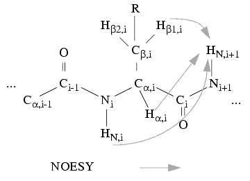
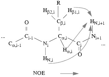
After spin-system delineation is complete, typically some spin systems remain that are not identified uniquely. Also, unique residue type identification is not always enough, since most biopolymers contain several copies of most residue types. These facts then necessitate the second step of sequence-specific resonance assignment, i.e., matching spin systems with specific residues. This is done through identification of NOE connectivities between spin systems corresponding to neighbor residues in the sequence.

Rigorous analysis of X-ray structures of globular proteins (Billeter et al. 1982) showed that several inter-residue distances are almost always small enough to yield cross peaks in a NOESY spectrum. These are, in particular: d_aN(i,i+1), d_bN(i,i+1), and d_NN(i,i+1). Usually d_aN(i+1,i) and d_bN(i+1,i) are not short enough. Therefore, these distances can be used to tie together stretches of spin systems by analyzing the NOE interactions between protons of different spin systems. If such stretches can be matched with stretches of residue sequence, sequence-specific assignment is achieved with a high level of confidence.

Since NMR data tend to be incomplete or ill-resolved, a systematic search of perfect assignments yields only partial results. One has to tolerate a significant amount of imperfection and use loose criteria in order to find a probable assignment. Even then, an exhaustive inspection of all possible solutions might become impossible within reasonable computation times. Optimization methods such as simulated annealing then provide a powerful alternative; all constraints are used to define an energy for the system, which is minimized according to careful schemes. No general tolerance has to be adjusted. The minimizer spontaneously allows imperfections where (and only where) no better solution can be found with the available data (just as it does if peaks are missing from a TOCSY pattern, or if NOEs or even residues are missing from a sequential assignment) (Morelle et al. 1994a, 1994b).

2D/3D homonuclear assignment strategy

The following steps were used by Eccles et al. (1991) for sequence-specific assignment of proteins based on homonuclear 2D spectra (DQF-COSY, TOCSY, and NOESY):

• Peak-pick all spectra.

• Identify ¹H spin systems of individual amino acid residues using systematic searching. Starting from the H_N-H_a cross peaks, the spin systems were disentangled based on DQF-COSY and TOCSY patterns and on the chemical shifts of key protons (chemical shift database). Each amino acid residue was represented by a single spin system, except for the aromatic side chains, asparagine and glutamine, which contain two separate spin systems. The substeps were:

a.   Start with the H_N-H_a cross peak in DQF-COSY.

b.   Identify all cross peaks belonging to this spin system using TOCSY (the alignment of COSY and TOCSY spectra may be rather poor - 0.03 ppm).

c.   Check all resulting groups against a database of 20 amino acid residues and score them.

• Assign individual spin systems to amino acid residues in the sequence. Using the sequential NOEs, polypeptide segments of variable length were identified and matched against the amino acid sequence of the molecule. This step can be automated, since all (except one, the Xxx-Pro) sequential NOEs (d_NN, d_aN, and d_bN) involve at least one amide proton.

a.   A search can be carried out along the w2 direction at the H_a, H_b,... resonances of each spin system (with an allowed uncertainty of 0.01 ppm) to find the corresponding H_N resonance of the sequential neighbor spin system. This can yield a list of NOE connectivities between the alpha, beta, and amide protons of each spin system and the amide proton of other spin systems.

b.   Uninterrupted pathways can be searched for, using the sequential NOEs and the amino acid sequence.

• These steps result in an assigned resonance list, which can be transferred to NOE peaks. This assigned NOE peak list can then be refined by using structure refinement and repeating the identifying and assigning steps several times.

For spin-system delineation you can use (besides 2D spectra) homonuclear 3D spectra such as the 3D TOCSY-TOCSY spectrum (Kleywegt et al. 1993). The spin system can be connected sequentially via 3D TOCSY-NOE or 3D NOE-NOE spectra.

3D/4D heteronuclear assignment strategy

Homonuclear experiments can have a great deal of spectral overlap, especially as the size of the molecule being studied increases. One way to alleviate the overlap problem is to use NMR-detectable heteronuclear atom labels such as carbon-13 and nitrogen-15 to singly or doubly label proteins or nucleic acids (some classic examples include Redfield et al. 1994, Hansen et al. 1994, Freund et al. 1994, Clubb et al. 1994, Anglister et al. 1994). Such isotopic labeling in common practice in the NMR community. Here, several methods of assigning singly or doubly labeled proteins are briefly described. The number of different 3D and 4D experiments available using labeled samples is virtually unlimited, so we limit our discussion here to the most widely utilized and implemented experiments. (For additional detail see Farmer et al. 1993, Sklenar et al. 1993, Marino et al. 1994, Legault et al. 1994.)

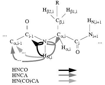
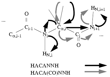
One of the first methods described in the literature used several combinations of double- and triple-resonance experiments to unravel the assignment for much bigger proteins than was possible earlier with homonuclear methods (Grzesiek et al. 1992). The steps involved can be summarized as follows:

• Measure HNCO, HN(CO)CA, HCACO, HNCA, NOESY-(¹⁵N)HMQC, TOCSY-(¹⁵N)HMQC, and HCCH-COSY for ¹⁵N and ¹³C doubly labelled proteins.

• Pick all peaks in all spectra.

a.   Some peaks could have been missing from some spectra. For example, if water presaturation was used to measure HNCA (which might have been necessary) the H_N protons, which were in fast exchange, would not give a signal when compared to HNCO.

b.   The typical peak halfwidth is 45-55 Hz for H_a and 35-45 Hz for C_a, therefore the peak positions were prone to ambiguities.

c.   Some spectra could have given extra peaks. For example, HNCA gave extra peaks for H_N,i-N_i-C_a,i-1, but this can be used in conjunction with HN(CO)CA. Special care was taken in automated assignment.

• Look through the HNCO list and find all H_N,i-N_i-C(O)_i-1 correlations.

• Compare the above list with HN(CO)CA, which also yielded (for each resonance triplet H_N,i-N_i-C(O)_i-1) the C_a,i-1 resonance. The extra peaks of HNCA could have also been used instead of or in addition to the above at this step to obtain the same information (that is, if it were known which ones were the extra peaks).

• Using the list of C_a and CO frequencies, search through the HCACO and find the possible corresponding H_a,i-1 resonance (or the set of such resonances).

• Search the HNCA, the TOCSY-(¹⁵N)-HMQC, and the NOESY-(¹⁵N)-HMQC spectra for H_N,i-1-N_i-1 resonance pairs from earlier assignments to the corresponding C_a,i-1 (in HNCA) H_a,i-1 (in TOCSY-NOESY) pair. This can give multiple possibilities due to severe overlap in the H_a/C_a region. The differences and similarities in the TOCSY-(¹⁵N)-HMQC and NOESY-(¹⁵N)-HMQC spectra could help with the overlap. For example, if there is a d_NN connectivity (because of helical structure), NOESY gives rise to signals for both H_N,i-1-N_i-1-H_N,i, H_N,i-1-N_i-H_N,i and H_N,i-1-N_i-1-H_a,i-1, while TOCSY results in H_N,i-1-N_i-1-H_a,i-1.

• Obtain the corresponding H_b/C_b pairs for the H_a/C_a pair via HCCH-COSY.

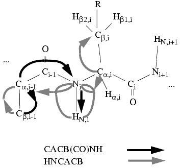
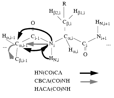
For smaller proteins you can use fewer triple-resonance experiments and still achieve good sequential assignment of the backbone. In particular, you can use a combination of two 3D triple-resonance experiments (Grzesiek and Bax 1992), which correlates the C_b, C_a, N, and H_N resonances of the ith and i-1^th residues using CBCANH or HNCACB and CACB(CO)NH experiments. Then the residue types can be identified using a database of C_a and C_b chemical shifts (Grzesiek and Bax 1993).

You can also choose to apply 4D methods using these steps. Although they are usually limited by spectrometer time, the information content of two 4D spectra can be very large. Ideally, for example, you can use a HNNCAHA or HACANHN experiment and a HACA(CO)NHN experiment to obtain a complete list of H_a,i, C_a,i, N_i, H_N,i, H_a,i-1, and C_a,i-1 resonances. From this list you can then construct a full sequential assignment of the backbone (Boucher et al. 1992a, 1992b, Constantine et al. 1993).

---

Assign building blocks

The Assign module includes several building blocks: the database, the visualization and analysis tools, and the automated algorithms.

The database consists of the data structures, which are built on the FELIX database management system. Using this Assign tool, you can keep all necessary information in a compact binary file, from which the specific entities can be exported in ASCII format. Also, FELIX provides spreadsheet capability, allowing you to view and, in certain cases, edit the entities.

The Assign database is structured in several layers. First you define a project entity, which is a container entity (i.e., it is at the top level and contains all information about the lower-level entities). The project entity, in which the assignment is carried out, then contains spectrum parameters (e.g., plot appearance, peaks, and spectra type description); spin-system information (patterns and frequencies, together with properties); sequence information (if any); the library of chemical shifts of residues; and various entities needed in the assignment procedure.

The following table lists the most important entities and symbols used in an Assign project:

Visualization and analysis tools are provided by the graphical user interface (GUI). Functionality in the Assign module is organized into several submenus. Menu items dealing with repetitive visualization tasks (e.g., changing plot type, redefining plot limits and plot parameters) are easily accessible at all times through icons at the top of the FELIX window. In addition, several commands that help the assignment process are mapped to the right mouse button (drawing frequencies, picking and removing peaks,and displaying correlated cursors). Menu items specific to Assign include tools for tiling patterns in different spectra, overlaying contour plots, easy access to strip plots, and displaying frequency lists from different sources on different spectra.

When working with multiple 3D/4D data sets at once, quick access to different spectra as well as coordinated navigation through 2D planes of different views of different spectra is crucial for successful assignment. Therefore multiple spectra can be connected in one, two, or three dimensions, letting you define which axes from which views are to be changed together when plot limits are changed. There is also the option, as mentioned above, to overlay multiple spectra in the same window.

Many automated algorithms that facilitate the sequential assignment strategy are found within the Collect Prototype Patterns, Frequency Clipboard/Compare Frequencies, Residue Type/Score Residue Type, Residue Type/Match Residue Type, Neighbor/Find Neighbor Via..., Sequential/Systematic Search, Sequential/Simulated Annealing, and Peak Assign/Autoassign Peaks menu items.

The prototype-pattern detection menu items serve as spin-system detection tools. FELIX currently has several methods for automatically detecting spin systems:

The 2D homonuclear systematic search algorithm performs the steps shown in the following figure.

• Depending on the method, collect the cross peaks in the defined seed area (in COSY, TOCSY, or both).

• Depending on the method, collect the cross peaks in the expansion area (in COSY, TOCSY, NOESY, or all).

• For every peak in the seed area, use the coordinates as the first two frequencies of a potential prototype pattern.

• Loop through all expansion peaks. If a peak is found for which exactly one frequency occurs in the new prototype pattern and the other does not, then this frequency is a candidate. The program scores and removes the candidate if the constraints are not satisfied.

• Sort the candidates by score, keeping the best ones.

• Start over at the beginning of the loop, unless: (a) there were no suitable candidates, (b) the prototype pattern now contains the maximum allowed frequencies, or (c) the maximum number of loops has been reached.

• Apply filters, if any. With filtering, prototype-pattern detection is made selective. That is, you can decide how many frequencies a valid prototype pattern should contain in various regions. Also, by defining the minimum and maximum number of frequencies that may be contained in a new prototype pattern, you can selectively detect spin systems (e.g., glycines and AMXs).

The 3D homonuclear spin-system detection algorithm can be used on a [J,J]-, a [J,NOE]-, or a [NOE,J]-type experiment and performs the steps in the following figure.

• Collect the cross peaks in the defined seed area. The pseudodiagonal peaks are left out of this set.

• Collect the cross peaks in the expansion area. The pseudodiagonal peaks are left out of this set.

• Use user-specified coordinates as the first two frequencies of a potential prototype pattern for every peak in the seed area.

• Loop through all expansion peaks. If the algorithm finds a peak in which exactly two frequencies occur in the new prototype pattern and the third frequency does not, this frequency is a candidate if its coordinate was set to be used. The algorithm scores and removes the candidate if the constraints are not satisfied.

• Sort the candidates by score, keeping the best ones.

• Start over at the top of the loop, unless: (a) there were no suitable candidates, (b) the prototype pattern now contains the maximum allowed frequencies, or (c) the maximum number of loops was reached.

• Apply filters, if any. With filtering, prototype pattern detection is made selective. That is, you can decide how many frequencies a valid prototype pattern should contain in different regions. Also, by defining the minimum and maximum number of frequencies that can be contained in a new prototype pattern, you can selectively detect spin systems (e.g., glycines and AMXs).

The 2D simulated annealing detection algorithm uses these steps:

• Use only half of the TOCSY or COSY spectra, for the sake of simplicity, no matter what the peak-picking file contains. The algorithm uses the half beneath the diagonal, except for the fingerprint region (w1>6 ppm, w2<6 ppm), for which the upper part is used to avoid the water signal. Then the selected peaks are reflected about the diagonal to yield complete symmetrical spectra.

• Attempt to assign peaks to a requested amino acid spin system, rather than recognizing patterns in the spectra. This system is defined from the usual shifts and correlations library as a list of requested TOCSY cross peaks. To reduce the space to be searched, the homonuclear TOCSY cross peaks are sorted according to frequency in several overlapping regions, each corresponding to one correlation (or a few equivalent ones) of a specific residue type. If the COSY spectrum is available, the TOCSY peaks are matched against it to further reduce the number of suitable peaks in each region. In addition, a natural-abundance ¹H-¹³C HSQC spectrum can be recorded to identify possible related carbon frequencies for each proton frequency and to use the powerful carbon chemical shift ranges as an additional constraint (Medvedeva et al. 1993). Each proton frequency is matched to a few HSQC cross peaks (one for each overlapping proton spin). The carbon chemical shift is very specific to amino acid type and spin, which allows you to reduce the number of possible regions for the corresponding TOCSY peak.

• Iteratively fill the pattern with these TOCSY peaks, using an adapted simulated annealing routine. The algorithm computes an energy at each step, which takes into account the relative alignment of the peaks in the motif. The program randomly chooses one cross peak among the unsatisfactory ones (empty, or misaligned peaks) and tries a permutation between the original peak and one from the adequate region in the TOCSY pool. Depending on the energy variation, the former peak might be released into the pool and the new one stored into the pattern, Eventually, the system converges to a pattern of consistently aligned peaks. A maximum number of missing peaks is tolerated, according to the specified amino acid type. Whenever the algorithm does not find enough aligned peaks, the pattern contains some empty (null) peaks. If the pattern ends up completely empty, it is not stored as a prototype pattern.

Assign implements several heteronuclear spin-system detection methods, which can be based on double- and triple-resonance experiments.

It is possible to use a ¹⁵N separated TOCSY experiment to collect spin systems starting on H_N and N frequencies of the pseudodiagonal peaks (i.e., ¹⁵N-H_N-H_N peaks). The algorithm is similar to the 3D homonuclear one, but you need to specify the dimension that the root frequency (i.e., the H_N) is in, and then all the frequencies are collected into spin systems that have peaks with the same H_N and N frequencies. A method for collecting spin systems starting with 2D peaks is also implemented. For this method, you need to provide a ¹⁵N-¹H HSQC and an ¹⁵N-HSQC-TOCSY spectra (certainly they can be HMQC, too).

Triple-resonance based spin-system detection algorithms are also provided in Assign. Particularly, you can use a combination of three 3D spectra - the HNCO, HN(CO)CA, and HNCA - and collect inter-residue spin systems or prototype patterns containing H_N,i-N_i-C_a,i-C_a,i-1-C_i-1 frequencies. Then during promotion to patterns, an automated routine can find the sequential neighboring systems and store the results as neighbor probabilities.

Similarly, you can use two triple-resonance 3D experiments - a CBCA(CO)NHN and a CBCANHN or HNNCACB - to collect prototype patterns containing H_N,i-N_i-C_a,i-C_b,i-C_a,i-1-C_b,i-1 frequencies, and a similar promotion can be carried out. Now you can also use the ¹⁵N-¹H HSQC spectrum to help collect the spin systems - mixing the information from heteronuclear double- and triple-resonance spectra.

In a similar method to that used in the previous example, you can collect spin systems in three triple-resonance experiments: HNCO, CBCANH, and CBCACO(N)H. This method results in spin systems containing: H_N,i-N_i-C_a,i-C_b,i-C_a,i-1-C_b,i-1-C_i-1.

It is possible to use an experiment to specifically find glycine spin systems (Wittekind 1993). A spin-system detection method is implemented in Assign for this, using the HNHA, CBCANH, and CBCA(CO)NH spectra.

Finally, you may use two 4D triple-resonance experiments - an HACA(CO)NHN and HACANHN - to automatically collect prototype patterns containing H_N,i-N_i-C_a,i-H_a,i-C_a,i-1-H_a,i-1 frequencies.

A visual tool is provided to allow you to quickly find the previously detected spin systems in multidimensional spectra and to verify them visually.

The Frequency Clipboard/Compare Frequencies menu item checks a frequency list against a set of patterns or prototype patterns. The algorithm finds how many "fuzzy similarities" (Kleywegt et al. 1989) are present between the current collection of frequencies and the frequencies in each pattern or prototype pattern. You can use this to decide whether a new frequency list constitutes a new pattern.

The residue-type matching and scoring of patterns helps in assigning frequencies in patterns to specific residues. For each frequency in a pattern, the match-type action calculates a delta value based on the library expectation values and standard deviations collected for each residue type (delta = [actual_shift_of_freq - expectation_value]/standard_deviation). The score-type action automatically matches patterns and residue types. The algorithm tries to find a matching frequency in the pattern. The best-matching frequency may lie no more than a given number of standard deviations away from the expectation value. If at least a certain number of atoms can be matched, a score is computed.

The Neighbor/Find Neighbor Via... menu items serve to find potential neighbor patterns through a 2D NOESY, a 3D [J,NOE], a 3D [NOE,NOE], or a ₁₅N-resolved NOESY spectrum. Therefore, this is the first step in sequence-specific assignment of patterns.

The algorithm consists of these steps:

• Loop through all NOE cross peaks. If one of the peak coordinates occurs in the selected set of frequencies of patterns considered and the other does not, the algorithm stores the latter as a candidate neighbor frequency.

• Store the candidates and search to ascertain which pattern contains the candidate frequency as root frequency. If such a pattern is found, this is a candidate neighbor pattern.

• Sort the candidate neighbor patterns and store them together with their scores.

FELIX implements a triple-resonance-neighbor-finding algorithm in the Neighbor/Find Neighbor Via 3D/4D menu item. This action works on a triple-resonance experiment (e.g., HN(CO)CA or CBCA(CO)NHN) which contains cross peaks connecting neighboring residues. The algorithms for each pattern look through the spectrum and try to find peaks that connect this pattern to, for example, the i-1^th residue. Then the sequential connectivity is set for the pattern that had the candidate frequency.

The Sequential/Systematic Search and Sequential/Simulated Annealing menu items find potential matches of patterns with the sequence of an unbranched biopolymer. This can be done using systematic search methodology through a recursive matching procedure or using simulated annealing. In the latter case, the program tries to assign a set of patterns to the primary sequence (or a requested segment of it) of the molecule using optimization techniques rather than systematic searching. Each step in the simulated annealing routine is a permutation between the pool of patterns and a residue in the sequence (initially filled with empty dummy residues and, optionally, some previously assigned residues) or between two stretches of residues tentatively assigned in the primary sequence. The energy is computed from previously determined residue-fit scores and neighbor information. Eventually, the results converge to a solution of low energy, which is unique in well defined parts of the sequence. However, when the data are inadequate, several runs of the program might yield locally different solutions.

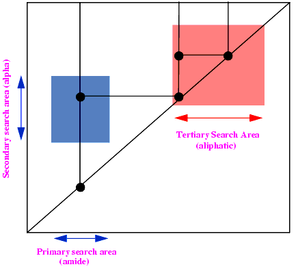
The Peak Assign/Autoassign Peaks menu item automatically assigns J or NOE peaks based on a set of assigned patterns, library, and molecule information. The patterns must have spectrum-specific shifts set for their resonances. The algorithm works as follows:

• Each peak's frequencies are compared against the assigned resonances of patterns.

• If candidate assignments are found, then the NOE connectivities are filtered against the provided distance cutoff (rejection cutoff), and the J connectivities are filtered against the J-step cutoff.

• If multiple candidate assignments remain:

a.   If one of the possible assignments has a distance connected to it that is shorter than the unambiguous cutoff and none of the others do, then this assignment is stored as a single assignment.

b.   If more than one of the possible assignments has a shorter distance than the unambiguous cutoff, or none do, and multiple assignment is requested, then these are stored as multiple possible assignments.

• If a single candidate assignment remains, it is stored as a single assignment.

• NOE distance-filtering is omitted if only one candidate assignment is present and a flag is set to not enforce distance cutoffs. This latter option should be used with caution, since it can lead to misassignment. However, it prevents you from including ambiguous structure information in the assignment if there is no good structural model yet.

---

Model

---

Calculation of theoretical nuclear Overhauser effects (NOEs)

A crucial part of the Model module is the calculation of the theoretical proton NOEs for a model structure. The basic physical principles underlying these calculations are described here.

Multi-spin relaxation

Multi-spin relaxation of a biomolecule in solution can be approximately described by the generalized Bloch equations (Boelens et al. 1988). In this approximation, the time development of the matrix of normalized cross-peak intensities A in a 2D NOE spectrum is described by a set of coupled differential equations (Ernst et al.1987, Keeler et al. 1984, Massefski et al. 1985, Dobson et al. 1982). First:

Eq. 5

which can be formally solved for a mixing time r_m as:

Eq. 6

where R is the relaxation matrix with:

Eq. 7

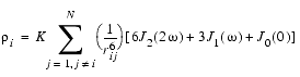
The relaxation rate constants in the dipolar cross-relaxation matrix for a rigid molecule with N protons are defined (Ernst et al. 1987, Dobson et al. 1982) by:

Eq. 8

and:

Eq. 9

where r_ij is the distance between protons i and j and K = 0.1 g4 (h/2p)². For isotropic tumbling of the molecule with a correlation time r_c, the spectral densities J_n (nw) take the simple form:

Eq. 10

where w is the Larmor frequency of the protons. The exponential matrix exp[-Rt_m] can be expanded in a power series:

Eq. 11

.

For sufficiently short mixing times, only the first two terms in Eq. 14 contribute appreciably, and the NOE intensity a_ij becomes s_ij ¥ t_m,which builds up linearly with the mixing time.

Alternatively, the matrix equations can be solved as:

Eq. 12

where l is the eigenvalue matrix obtained after diagonalization of R, and X is the matrix of eigenvectors:

Eq. 13

Therefore, given a molecular model, the NOE matrix can be calculated from the relaxation matrix for each mixing time t_m of a 2D NOE experiment, and the buildup of NOE intensities in a time series can be obtained.

The reverse procedure is also possible, although so far it has only been applied to systems with chemical exchange between a small number of sites (Massefski et al. 1985, Dobson et al. 1982). When the complete NOE matrix A is known, the relaxation matrix R can be obtained by diagonalizing the NOE matrix (Ernst et al. 1987, Olejniczak et al. 1986):

Eq. 14

Eq. 15

Thus theoretically, matrix R can be obtained from one 2D NOE experiment performed at a suitably chosen mixing time. In practice, averaging over a series of t_m values is more accurate.

Additional detail on the full treatment of dipolar spin relaxation of spin networks in the presence of internal motions appear in Boelens et al. (1988, 1989), Koning (1990), and references cited therein.

Efficient calculation of NOEs

The Model module of FELIX offers a very efficient method for computation of NOEs.

The NOE matrix is related to the rate matrix as described in Eq. 11. In principle, one can calculate NOEs exactly by diagonalization (Eq. 12). Unfortunately, the computational load of diagonalization is too demanding (O(N 3)), to allow for fast back-calculation. Thus, one must seek an alternative method of evaluating NOEs. We present a method here which utilizes the general properties of the matrix exponential operator and the distance dependence of the rate matrix.

As mentioned earlier, the NOE matrix is related to the rate matrix as follows.

If t_m is sufficiently small, you can ignore the higher-order terms and approximate the NOE matrix by the linear term:

Eq. 16

The problem is then to obtain the NOEs at longer mixing times. The multiplicative properties of the matrix exponential are the key:

Eq. 17

If the mixing time t is broken down into 2ⁿ smaller times steps s, such that t = s2n, then you have:

Eq. 18

which leads to:

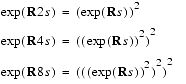
Eq. 19

Thus in n steps of repeated matrix squaring (or doubling in the time parameter - the notation of the method used in FELIX is matrix doubling and refers to this procedure), we arrive at (exp (R · t)) from (exp (R · (t/2ⁿ)). For example, to get to t_m at 128 ms from 1 ms, we only need to do 7 matrix-squaring operations. The formula in Eq. 16 allows one to bootstrap from NOEs at a small mixing time, where a linear approximation (Eq. 16) is justified. To truly make such an scheme efficient, one must optimize the performance of the matrix multiplication involved. To this end, make use of the distance dependence of the rate matrix:

Eq. 20

The inverse power-of-six behavior implies that the rate drops off extremely rapidly with distance. Thus, for most practical applications, one can impose a cutoff distance beyond which R is assumed to be zero. This further implies that the resulting R matrix is sparse. The matrix multiplications involved can then exploit the sparsity of the rate matrix (and the resultant NOE matrices) to gain substantially in efficiency.

Methyl group rotation and ring flipping

The application of a general theory of spin relaxation to biological molecules is usually hindered by the lack of a complete description of the molecular motions over a sufficiently long time scale. You can nevertheless account for certain types of internal motions such as methyl rotations and ring flipping. Remember that, although any one particular model for such motions would not be perfectly satisfactory, it is nevertheless important to use more physically based models that involve fewer adjustable parameters and are rigorously derived from well defined assumptions. Thus for methyl rotations and ring flips, we adopt the jump models as proposed by Tropp (1980). We further assume that methyl rotations occur over three sites and on a time scale much shorter the overall tumbling time of the molecule. For ring flips, the jumps are assumed to occur over two states (180° flips) and on a time scale much slower than the tumbling time. The relaxation rates are then modified to include the contributions from the various jump states. For further details see Yip and Case (1991). An important feature of the jump models that we assume here is that no additional parameter is in the relaxation matrix other than those already used by the rigid isotropic tumbling model.

---

Autoscreen module

---

Introduction

NMR techniques for characterization of protein-ligand interactions are being widely used in rational drug design. As an example, the SAR by NMR strategy, devised by the Fesik group at Abbott Laboratories (Shuker et al. 1996; Hajduk et al. 1997), consists of the following general steps:

1.   First, a library of small molecules is screened for binding to an ¹⁵N-labeled protein. If a molecule binds to the protein, it alters the local chemical environment and thereby cause changes in the chemical shifts of nuclei in the protein's binding site. Such changes are detected in HSQC spectra acquired in the presence and absence of added ligand.

2.   Once initial ligands are identified, analogs are screened and binding constants are obtained in order to optimize the interactions with the protein.

3.   Next, the 3D structure of the protein complexed with the ligands is obtained, and linked compounds are synthesized based on this structural information.

The Autoscreen module of FELIX automatically characterizes the protein-ligand interactions by identifying the changes between the reference and test spectra. With Autoscreen you can organize the project, process and score the 2D test spectra, and identify high-affinity ligands. For the above SAR by NMR steps, it offers help for the first two steps.

---

Autoscreen strategy

Autoscreen analysis of 2D ¹⁵N-HSQC data consists of the following general steps:

1.   Organizing HSQC experimental data into a project. The data can be FID raw data from various spectrometers or processed data. An experiment can be associated with one or more molecules.

2.   If raw data are used, process the control (or reference) spectrum. The same processing methods and parameters are remembered for processing all other spectra. Otherwise, if processed data are used, designate one of them as the control.

3.   If available, input the peaks and assignments of the control spectrum. Otherwise, do peak picking and resonance assignment in the 2D and Assign modules, respectively.

4.   Process and score the test spectra.

5.   Cluster the experiments based on their displaced peaks and identify binding subsites. Export the results for QSAR study, fitting K_d, etc.

---

Scoring

A crucial step in using the Autoscreen module is scoring of the test spectra against the control spectrum. This consists of the following steps:

1.   Pick peaks in the test spectrum.

2.   Match test peaks to control peaks based on chemical shifts and peak shapes, and then score the experiment based on the displacements between the matched peak pairs.

3.   Add penalties for the unmatched control and test peaks to the score.

The underlying principles are explained in the following sections.

Basics

The prerequisites for a test peak to be matched to a control peak are Eqs. 21-23:

Eq. 21

Eq. 22

Eq. 23

where DH is the absolute displacement of the ¹H chemical shift between the test peak and the control peak, maxDH the upper limit of this ¹H displacement, DN the absolute displacement of the ¹⁵N chemical shift, maxDN the upper limit of the ¹⁵N displacement, S the shape similarity between the test peak and the control peak, and minS the lower limit of the shape similarity.

The test in Eq. 23 is applied when you choose to consider the shape of peaks. You can choose to define the shape similarity S as the product of the similarities of the peak widths and intensity:

Eq. 24

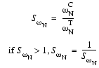
where S_wH, the similarity of peak widths along the ¹H dimension, is calculated based on the width of the control peak wC_H and the width of the test peak wT_H along the ¹H dimension:

Eq. 25

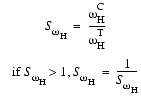
Analogously, S_wN, the similarity of peak widths along the ¹⁵N dimension, is calculated based on the width of the control peak wC_N and the width of the test peak wT_Nalong the ¹⁵N dimension:

Eq. 26

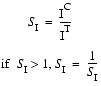
SI, the similarity of peak intensities, is calculated based on the peak heights of the control peak I^C and of the test peak I^T:

Eq. 27

If a test peak is matched to a control peak, its contribution to the score of the experiment is:

Eq. 28

where a and b are the weights of the ¹H and ¹⁵N chemical shifts, respectively.

A control peak that does not match any test peak contributes a penalty c' (default is 0.6) to the score. The score of an experiment is hence the sum of the contributions of all matched and unmatched control peaks:

Eq. 29

Sometimes some of the test peaks do not match any control peak. Although most unmatched test peaks are noise, any that are legitimate peaks can, if you choose to, contribute to the score such that:

Eq. 30

where cð is the penalty for each unmatched test peak.

Normally, the contribution of peaks with too-small displacements are ignored, namely:

Eq. 31

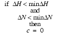
where minDH and minDN are the lower limits of the ¹H and ¹⁵N displacements, respectively.

In practice you can change the weight of some control peaks to hide or highlight their contributions. In this way the reported score becomes:

Eq. 32

where W is the weight of each control peak. Since test peaks are automatically picked on the fly, you cannot specify weights for them. Furthermore, although they contribute to the score, unmatched test peaks are not stored in the database as other peaks are.

Except in the simplest case, Eqs. 21-23 do not guarantee an unambiguous mapping of all test peaks to control peaks. Based on the assumptions that only a small portion of the peaks are displaced and that most peaks retain their locations and shapes in the test spectrum, Autoscreen assumes that the mapping that has a global-minimum value C as defined in Eq. 29 is the true mapping.

Intelligent peak picking in test spectra

Peak picking in test spectra is done on the fly during scoring, i.e., you have no chance to optimize the picked peaks, hence the quality of the picked peaks is one of the key factors for successful scoring. Although most of the peak-picking parameters should remain identical to those used for peak picking in the control spectrum, the threshold may need to be adjusted for differences in sample concentrations.

Autoscreen first determines a peak-picking area, which is the minimum rectangle that includes all the control peaks plus margins of maxDH and maxDN in the D1 and D2 dimensions, respectively.

Autoscreen provides three ways of defining the threshold for peak picking: Automatic, Control, and Define. If the default setting (Automatic) is selected, an initial threshold is automatically calculated, and then the threshold is raised or lowered according to the following rules for each test spectrum:

1.   If the number of test peaks is fewer than 1.1 times the number of control peaks, lower the threshold.

2.   Otherwise, for each control peak, the test peaks that meet the criteria of Eqs. 21-23 are taken as candidate matches to the control peak. If over 10% of control peaks do not have a candidate match, lower the threshold.

3.   Otherwise, if the number of test peaks is greater than 1.5 times the number of control peaks and each control peak has more than 3.0 candidate matches on average, raise the threshold.

No more than seven adjustment loops are performed.

If Control or Define is selected for the threshold method, the same threshold as that used for the control spectrum or a user-defined threshold is applied to all test spectra, respectively, and no automatic adjustment of thresholds is done.

Mapping control peaks to test peaks

For each control peak, the contributions of those test peaks that meet the criteria of Eqs. 21-23 are calculated using Eq. 28. These test peaks are sorted in ascending order of c, and the first four are retained as candidate matches. At this stage, similarities in peak heights (SI) are not used in Eq. 24, since the intensity level may be different between the control and test spectra.

To normalize the intensity level of the test spectrum, an intensity ratio IR is calculated as follows:

Eq. 33

where ÂIC is the sum of peak heights for all control peaks that have at least one candidate match, and ÂIT is the sum of peak heights of the first candidate matches to all control peaks. The peak heights of the test peaks are then normalized by multiplying by IR.

Next, the list of candidate matches is updated by including the peak intensity in Eq. 24.

The remaining task is to choose one or no test peak for each control peak, so that the sum of contributions (Eq. 29) is minimal. Some control peaks may not match any test peak, and such unmatched control peaks also contribute to the score.

Autoscreen provides two alternative methods for searching the mapping to find a global minimum for Eq. 29.

The first is a depth-first tree-search method. This deterministic method, in principle, should always find the true minimum, but in practice it may be too slow for complex spectra. Several heuristic methods are used to enhance its efficiency, so that, for normal spectra, satisfactory results are obtained in a few seconds. By default, the total CPU time is limited to 10 seconds although you can change this.

Another method is simulated annealing, a stochastic method that efficiently lowers the score (or energy) to or close to the global minimum. This method is recommended for very complicated spectra where tree searching does not give satisfactory results in a reasonable amount of CPU time.

Unmatched peaks

There are many possible reasons for a control peak not to match any test peak. For example, if the upper limits for peak matching are set to too low a value, a peak that is shifted very far will not find its match. More often, two well separated peaks in the control spectrum become overlapped in the test spectrum. When this happens, only one test peak is picked, leading to one of the control peaks' being unmatched.

To unravel the overlapping test peaks in the latter case, Autoscreen fits such unmatched control peaks to the test spectrum using a local optimization method (see Peaks/Optimize in Chapter 4., Processing, visualization, and analysis interface (1D/2D/ND) in the FELIX User Guide.) All unmatched control peaks, together with those neighboring control peaks that lie closer than four times their peak width to the unmatched control peaks, are fitted to the test spectrum with only the peak centers optimized. This process is iterated up to three times or until the change in the penalty is less than 5%. Next, the widths of these peaks are optimized for one iteration.

For each optimized peak, its equivalent peak height in the test spectrum is normalized using the intensity ratio, as for other test peaks. Then the optimized peak is matched to the original control peak to see if the conditions in Eqs. 21-23 are met. If this is successful, the contribution is calculated using Eq. 28. Otherwise, the control peak remains unmatched and its penalty is added to the score according to Eq. 29.

The fitting of unmatched control peaks to the test peaks is done only when the percentage of unmatched control peaks is below a certain threshold (default = 40%). If too many control peaks are not matched, this usually means that the spectrum is corrupted, and the fitting is not done. A corrupt spectrum usually has a score significantly higher than a normal spectrum, because of the contribution of unmatched control and test peaks.

Test peaks that are not matched to a control peak are usually noise, but they can also be real peaks corresponding to unwanted control peaks (e.g., the side-chain amide peaks are usually excluded from the control peaks), or to a control peak that was not noticed in the control spectrum because of peak overlap or other reasons. A legitimate test peak that was not observed in the control spectrum but that is picked in the test spectrum should contribute to the score.

Therefore, from all the unmatched test peaks, Autoscreen identifies legitimate test peaks based on their chemical shifts and peak shapes. If you choose to use the chemical-shift constraint, then only those peaks that are displaced less than maxDH and maxDN (in the ¹H and ¹⁵N dimensions, respectively) with respect to their closest control peaks are considered. Next, the peak widths and heights of all the matched test peaks are analyzed statistically. At this point, an unmatched test peak is considered legitimate if its peak widths (wH and wN) and peak height (I) meet the following criteria:

Eq. 34

Eq. 35

Eq. 36

where , , and are the average values of the peak width along the ¹H dimension, the peak width along the ¹⁵N dimension, and the peak height, respectively; sH, sN, and sI are the standard deviations of the peak width along the ¹H dimension, the peak width along the ¹⁵N dimension, and the peak height, respectively; and n is a user-defined coefficient (default value is 2.0).

By default, each unmatched test peak contributes a penalty of 0.20 to the score, though you can always change this parameter. This penalty is set smaller than that for an unmatched control peak, because you usually have a better chance to refine the control peaks based on the assignment. The test peaks, on the other hand, are automatically picked so are usually less reliable.

Presently, unmatched test peaks are only reported to you in the text window and in a log file, but not saved in the database like other peaks.

Table of scoring parameters

The Autoscreen/Setup Scoring menu item (see Chapter 8., Autoscreen user interface) allows you to change or verify the parameters used for scoring. The following table correlates these parameter names with the symbols and terms mentioned in this chapter, for your convenience.

Table 1. Meanings of Autoscreen scoring parameters 

Parameter	Options	Default	Symbol or meaning
Peak Displacement Limits (ppm)
	D1 Minimum	0.02	minDH in Eq. 31.
	D1 Maximum	0.13	maxDH in Eq. 21.
	D2 Minimum	0.2	minDN in Eq. 31.
	D2 Maximum	0.8	maxDN in Eq. 22.
Scale Factors
	D1	1.0	a in Eq. 28.
	D2	0.2	b in Eq. 28.
Threshold Methods		Automatic	Method for determining peak-picking threshold.
Use Peak Widths		Yes	Match peak width?
Use Peak Heights		Yes	Match peak intensity?
Minimum Shape Similarity		0.05	minS in Eq. 23.
Search Method		Tree Search	Method to search for the global minimum. Options are Tree Search and Simulated Annealing.
CPU Time Limit		10	Maximum CPU time (seconds) to spend searching the global minimum. Used only when Tree Search is selected.
Unmatched Control Peaks
	Fit to Test	Yes	Fit unmatched control peaks to test spectrum?
	Maximum	40	Upper limit of unmatched control peaks, above which the spectrum is regarded as corrupt and no fitting is done.
	Penalty	0.6	Penalty for an unmatched control peak (c' in Eq. 29).
Unmatched Test Peaks
	Selection	Close to Control Peaks	Method for identifying unmatched test peaks.
	Num.of RMSD	2	n in Eqs. 34-36.
	Penalty	0.2	Penalty for an unmatched test peak - cð in Eq. 30.